Object Detection and Getting Started with LiDAR
In this blog post, I will be going over some updates regarding our object detection algorithm and where we are currently at. After that, I will go over the current LiDAR bench testing setup and our next steps.
Object Detection
As discussed in Andrew’s post regarding our vision pipeline, we have decided to perform cone detection with neural networks. Since this is already a well-researched field, there are many existing networks and implementations which we can adapt and use for our project.
Model Selection
Here, the various different image detection networks will be discussed and compared. The comparison metrics such as mAP (mean average precision) and IOU (intersection over union) will be used for performance evaluation. The main contender in this section will be YOLO (You Only Look Once).
While YOLOv3 was the definitely the state-of-the-art object detection network when it was first released in 2018. Since then various new networks have been released, some with better detection results, while others are optimised for even faster inference speed.
The table below shows a small list of detector networks considered. While this list is not comprehensive by any means, various new networks have been added as an attempt to filter out a worthy successor to the original YOLOv3. In particular, csresnext50-panet-spp-optimal network demonstrates significant improvements over the original YOLOv3 while still delivering near real-time performance at 35FPS.
Other network architectures improves upon the original YOLOv3 network by integrating spatial pyramid pooling (SPP) to the original network, which results in better feature extractions. On the other hand, the idea of training a sparse network and pruning near-zero weights were applied on SlimYOLOv3 to achieve similar network performance with a fraction of the original amount of network weights (the pruning threshold can be defined specifically, paper was presented with 50%, 90% and 95%). CornetNet takes a different approach to object detection, as it detect object bounding box as a pair of key points and was able to achieve impressive results over the existing one-stage detectors.
| Name | mAP | AP50 | AP small | FPS | BFLOPS |
|---|---|---|---|---|---|
| YOLOv3 (416 x 416) | 31.0 | 55.3 | 15.2 | 46 | 65.9 |
| YOLOv3 (608 x 608) | 33.0 | 57.9 | 18.3 | 25.6 | 140.7 |
| YOLOv3-SPP | 36.2 | 60.6 | 20.6 | 30 | 141.5 |
| csresnext50-panet-spp-optimal (608 x 608) | 38.4 | 65.4 | 22.1 | 35 | 100.5 |
| CornetNet-Squeeze | 34.4 | - | 13.7 | 30.3 | - |
| SlimYOLOv3-SPP-50 (416 x 416) | NA | NA | NA | 67 | - |
The comparison metrics used are:
- mAP (mean average precision)
- AP50 (mAP at 50% IOU)
- AP small (average precision for small objects with area smaller than 32 x 32 pixels)
- FPS (frames per second) on a GTX 1080 Ti
- BFLOPs (billions of floating point operations)
- MS COCO dataset is used to training and validation
- Note: In the paper, SlimYOLOv3 was trained on the VisDrone2018-Det benchmark dataset, hence no data is available.
- For a more detailed table on existing object detection networks, please see the CSPNet paper, which provides a really comprehensive overview of existing networks and their performance.
In the end, no single network was chosen for the project. Instead, various different networks would be trained to validate their actual performance on our own dataset. After that, we would have a better idea on what is the most suitable network for this particular project.
Training and Validation
We started off by training a proof-of-concept detector by using a subset of the existing open-source traffic cone dataset from MIT Driverless, and also some images which we have taken during a recent track day event.
class_id = 0, name = blue   cone, ap = 93.21%   	 (TP = 291, FP = 55)
class_id = 1, name = orange cone, ap = 90.15%   	 (TP = 176, FP = 22)
class_id = 2, name = yellow cone, ap = 92.41%   	 (TP = 366, FP = 41)
  for conf_thresh = 0.25, precision = 0.88, recall = 0.90, F1-score = 0.89
  for conf_thresh = 0.25, TP = 833, FP = 118, FN = 97, average IoU = 69.26 %
  IoU threshold = 50 %, used Area-Under-Curve for each unique Recall
  mean average precision (mAP@0.50) = 0.919253, or 91.93 %
However, soon after the proof-of-concept detector was trained, I realised that the the MIT dataset also came with the corresponding data labels for all the cones in the images. The only downside is that the labels they provide is for one-class only, which means that the labels do not differentiate between blue, yellow or orange cones. See below for a brief summary of the validation done on the best weights for this one-class setup.
detections_count = 24110, unique_truth_count = 12891
class_id = 0, name = traffic cone, ap = 79.47%           (TP = 10386, FP = 3092)

  for conf_thresh = 0.25, precision = 0.77, recall = 0.81, F1-score = 0.79
  for conf_thresh = 0.25, TP = 10386, FP = 3092, FN = 2505, average IoU = 59.04 %

  IoU threshold = 50 %, used Area-Under-Curve for each unique Recall
  mean average precision (mAP@0.50) = 0.794682, or 79.47 %
Total Detection Time: 309 Seconds
Getting Started with LiDAR
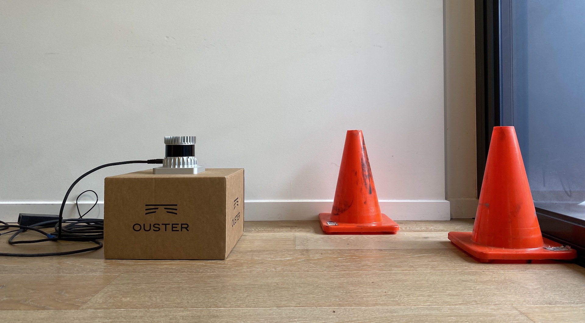
Shown below is our indoor LiDAR bench testing setup. Fortunately, we were able to retrieve the required hardware and testing equipment (mainly the 2 orange cones) so that we can better validate and test our proposed LiDAR pipeline.
The OS1-64 LiDAR is fairly straightforward to setup and easy to connect. The main things to take note is that you would need to udpate the wired network setting to manual and change some settings for IPv4.


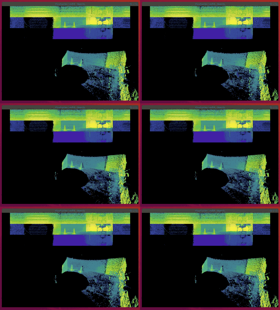
From the figure above, we can clearly see that the LiDAR can easily pick up the two orange traffic cones. However, the output point clouds do seem quite noisy as they visibly “jump around”.
Point Cloud Processing Pipeline

The first part regarding point cloud un-distortion is not implemented yet, but we would most likely require a simple testbed and an outdoor environment to properly test this. However, we can still rely on the Gazebo simulated LiDAR to conduct some initial testing.
Currently, we are working on the ground plane segmentation which can potentially be done with the help of PCL and PDAL point cloud processing libraries.
Once that part is done, we need to:
- cluster the remaining points
- reconstruct neighbouring points which may have been removed during segmentation
- filter our clusters which have too few points remaining (this threshold will depend on LiDAR resolution and distance to cone)
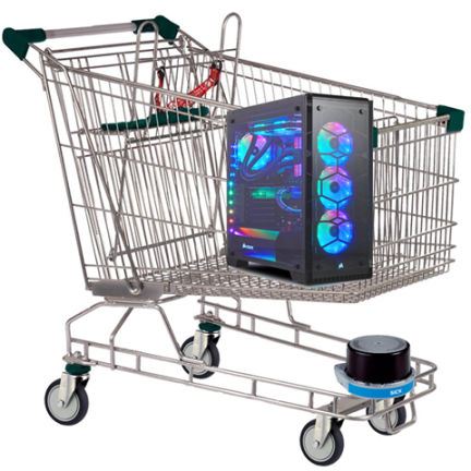
Shown below is a potential test bed for the perception subsystem. This was recommended by the Monash Driverless Team as it is really flexible, and all the sensors can be mounted in similar heights and locations as they would on the actual car. The main thing is that we would need to add air-filled tyres which should reduce the bumpiness and ensure the sensor data can be collected smoothly.
